|
A note about this publication:
The analysis performed for this study was done using Radio Mobile version 9.5.4. As with version 6.5.6 a change in the free space loss calculation was done, the presented analysis results will differ in dB's from a analysis performed with a newer version of Radio Mobile.
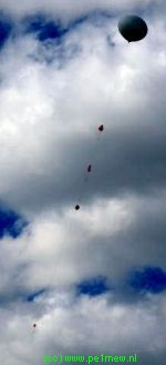
Each year in the Netherlands a group of radio amateurs launches a weather balloon that carries some amateur radio equipment. The equipment in 2009 was a VHF beacon, a UHF-VHF FM Cross band transponder, and a ATV transmitter on 13cm with a camera that is taking pictures from the ground.
The main purpose is to have a fox-hunt (ARDF) where over 20 groups of radio amateurs from all over the Netherlands chase the balloon to find it first. Secondary the balloon hunt encourages radio amateurs to develop and build receiver systems and antenna arrays for direction finding.
Third but not the least is that the balloon enables radio amateurs to do research on RF propagation.
This article will describe some measurements and investigations about radio propagation for Air to ground communication on VHF.
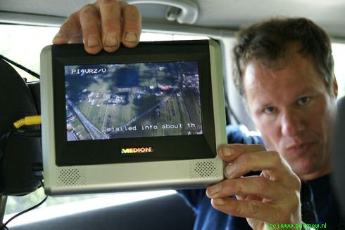
ATV reception minutes after launch |
2008 launch |
How the idea started
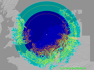
In the preparations to the balloon launch I simulated the coverage of the balloon at a altitude of 24 Km using Radio Mobile.Then I compared the simulated RF coverage with the visual coverage coverage.
Click on the image to view the full size image. |
There results of this analysis meets the expectation as the radio coverage (light and dark blue) is bigger than the visual coverage(Yellow and Orange).
In the simulation the balloon was elevated above the launch site of the Dutch Meteorology Institute (KNMI) at the Bilt at heights of 10.000 and 20.000meters.
Each hight is displayed using it's own colours:
At 20 Km: Light blue = radio coverage, Yellow line is visual coverage. At 10 Km: Dark blue = radio coverage, Orange line is visual coverage.
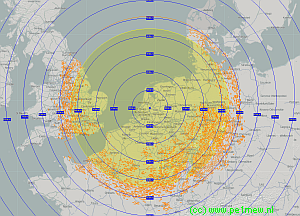
In the initial analysis a power of 1Watt was used at the balloon transmitter. Now the real power of the balloon was required and a link budget was set-up. (See below) |
Click on the image to view the full sizeimage. |
When the real power was applied to the simulation it was found that due to the low power of the balloon the radio coverage of the balloon was less than the visual coverage. If the balloon should have 3 dB more Erp power the radio coverage will meet the visual coverage boundary's.
Be aware that these radio coverage analysis ware perfomed with the ITM model using Mobile mode of variability with time probability of 98% and situation probability of 50%. This is much more than a radio amateur expects!. See 'Networkproperties > Parameters'.
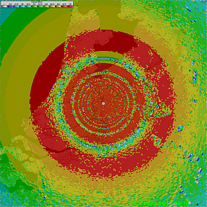
To estimate the range of the balloon, coverage circles have been added to the balloon in Radio Mobile. For this the function 'Draw rings' is used. |
Click on the image to view the full size image. |
After this initial success, simulation changed to the to be expected coverage of the balloon. When analysing the results confusion struck.
It was observed that from a altitude of 1000 meters these rings appear in the coverage analysis and that the position of the ring varies with the height of the balloon. It was also found that these dips have a depth of over 30dB.
After investigation the possible causes it was found to be most likely that ground reflections may cause this effect.
In Radio Mobile the model can calculate multipath fading as a part of the model. This part is called 'Propagation mode' and can be found in 'Network properties > Style'.
This type of fading should be categorised as slow-fading for the reason that Radio Mobile cannot simulate multipath fading in urban environment as it lacks the database for that purpose. |
The model in Radio Mobile can be set to calculate the influence of the reflected wave in 3 ways:
- Dot not use the reflected wave. When there is line of sight this estimates Free space loss.
- Include the effect of the reflected wave in a 'normal way'
- Include the effect of the reflected wave in 'Interference mode'
As these 3 settings are the only parameters that can be set in Radio Mobile this was the range in which the model can be tuned.
Results of changing the model
To determine the effect of the various settings all 3 settings have been used in a scenario where a balloon is launched and analysed at 500 meter intervals. The following animating images display the results in various modes.
 |
This analysis is performed not using the reflected wave. The result seems similar to Line Of sight.
By gaining more height with respect to a receiving station the distance from transmitter to receiver increases and so the path loss. |
 |
This analysis is performed while including the reflected (ground) wave in a 'normal way'.
|
 |
This analysis is performed while including the reflected (ground) wave in a 'Interferenced way'. |
The different animations show the effect on the received signal strength by a normal amateurradio station.
The Question
After this observation the main questions are:
- what to believe?
- How accurate is the model in Radio Mobile when used in air to ground communications?
- Which setting do I have to use to obtain accurate results
Required measurements
In the weeks before the balloon launch the idea was grown to perform two measurements using logging equipment to log the received RSSI at the two locations. The aim was to observe the fading signals of the balloon in the downlink and so reproduce the simulated behaviour.
There for at two amateur radio stations Spectrum analysers have been set up to record the received signal from the balloon at 2 meters. The stations are representative for a typical amateur radio station. Both have a omni antenna at the rooftop at about 10 meters.
The spectrum analysers(both R&S FSP) have been configured in zero span at the beacon frequency and tracing the frequency at a interval of one second. The traces ware recorded using a small program that is issued byR&S: Tracerec. Tracerec can be downloaded from the R&S internet website. This program 'tracerec' runs on a pc and is connected to the FSP over a Ethernet connection. The program records in 'ascii' mode a full trace in 500 points in a text file.
The captured data will be aggregated to be analysed afterwards.
Description of the measurement locations
For the link budget a recap of both stations.
The exact location is used in the analysis but not displayed in thisarticle.
PE1MEW
Location:JO22XE
Antenna: J-antenna
Antenna gain: x dB Gain
Antenna polarisation: vertical
Antenna height:10 meters
Cable type: RG213
Cable length: 10meters
R&S Spectrum analyser FSP |
 |
PE1RYY
Location: JO22KE
Antenna: GP-95
Antenna gain: x dB Gain
Antenna polarisation: vertical
Antenna height: 10 meters
Cable type: aircom plus
Cable length: 7 meters
R&S Spectrum analyser FSP |
- |
Description of the balloon
The balloon payload is using low power transmitters. This is because reduction of weight is one elementary activities in balloon missions like these.
As a reference to the other parts of this article you find the technical details of the balloon payload below.
| Overview of the systems (more info see the website) |
2 meter beacon.
Downlink:
Frequency 145.450 MHz
power 100milliwatts
Antenna: Horizontal dipole |
FM transponder.
Downlink:
Frequency: 145.425 MHz
Power:100 milliwatts
Uplink:
Frequency: 432.550 MHz
RX Sesitivity (assumend) -120 dBm @ 12 dB Sinad
Antenna: Horizontal dipole. |
ATV Transmitter.
Downlink:
Frequency: 24xx.xxx MHz
Power: 1Watt
Antenna: 4 single-8 antenna's combined together. |
This information will be referred to as they are part of the link budget.
The different antenna scan be seen on the image on the right. |
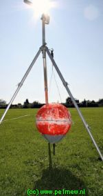
Baloon Payload beforelaunch |
The Red ball holds the CCTV Camera, ATV transmitter, and 2 meter beacon. Th grey triangular shape on the bottom of the red ball is the ATV antenna. The 2 meter antenna are 2 pices of copper wire that together form a dipole antenna.
Measurements
The was started before the balloon launch as both hams ware chasing the balloon as well.
After the return home the measurement was stopped at PE1MEW and at PE1RYY the measurement software was crashed but the data was not lost. At PE1RYY the log file was 27 MB and at PE1MEW 192MB.
When both files have been analysed for correlation it was observed that the spectrum analysers and the used PC's had different clock settings and it was found impossible to shift the PE1MEW log file in time to be able to make a accurate analysis onthe data. Therefore the PE1MEW data was dropped and the focus was on the PE1RYY data.
Also we experienced serious problems in aggregating and post processing data of this size in a Windows environment. The Office suite is simply not capable of handling such big data sets. There for we prepared the data in Notepad++ before imported in Excel or Access.
Balloon flight data
The flight data was provided by the launch crew of the balloon.
The GPS data holds Time, Latitude, Longitude (inWGS84), and Altitude (in Meters). The flight data has 156points.
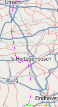
The flight data was in NMEA GGA datagrams($GPGGA) and was converted in to a line object file using Excel. This method is described in 'How to > Working with objects > Convert points to line objects'. The result of this process is put in to 3 different files.
All 3 files can be downloaded for analysis or as a example:
The Line object file is also required for analysis of the propagation model later.
For the purpose of verification the line object file is created and plotted in Radio Mobile. The result can be seen on the right side.
See the purple line.
Time is the only correlation to the measurement data. So the flight data was also timestamped. |
 |
Post processing
The dataset of PE1RYY is prepared and converted into Excel format.
The original data set has lines on which each line holds 501 RSSI values in dBm.
The Sweep time was set at 500 milliseconds and the delay capture time was set at 1Second.
Therefore the sweeps in zero span registered are at a1.5 Second interval at average.
Disadvantage of using Excel is the limitation of 255 columns and 64.000 lines. Because of this we lost half the data of the 500 ms sweep.
The dataset from PE1RYY was similar to the flight data time stamped.
Because the measurement data has a large variation the data was averaged over a minute. In this minute at a average rise speed of 6 m/S the altitude increase is proximately 360 meters.
Analysis of the flight data
The flight data is looked into out of curiosity. It was observed that the available data does not have much points compared to the available measurement data.
From the flight data it is observed that the balloon has a continues rise speed until the moment on which the weather balloon exploded. From that moment on anon-linear falling speed is recognised. This might be caused by 'vacuum' at high altitude.
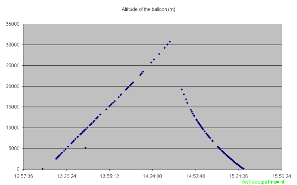
Balloon altitude over time graph
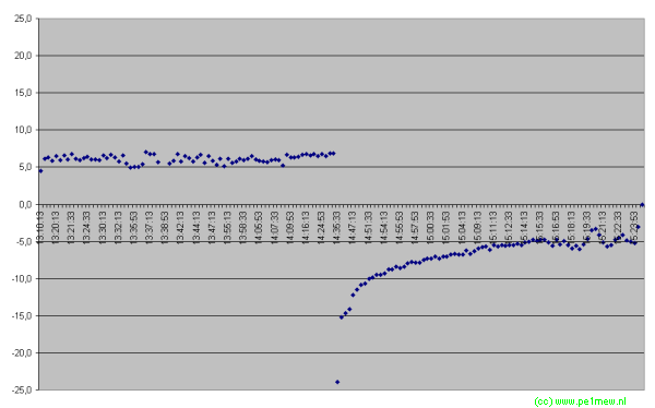
Balloon rise- and fall speed graph
Analysis of the measurement data
The RSSI measurements at PE1RYY are displayed in the following graph. The blue line is the raw 1,5 second interval RSSI value. The purple line is the one minute averaged RSSI value.
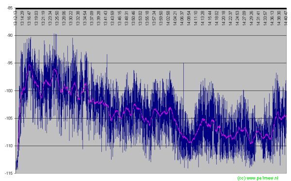
Click on the graph for the full size image.
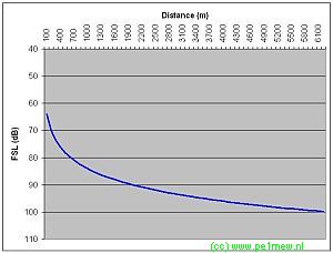
The average line (purple) shows the slow decrease of signal strength that fits with the rising of the balloon as the distance between the receiver and transmitter increases. This trend in the effect is caused by variation in Frees Space Loss (FSL). As a demonstration a Free space loss curve is displayed on the right.
The variation in the averaged signal however can be caused by ground reflections. More about this later in this article.
The variation in the blue line is at a maximum +/- 10 dB or 20 dB. This might be caused by the rotation of the balloon payload and the dipole antenna but cannot be verified because only 1/3 of the time the receiver is registered. |
 |
As the polarisation of the balloon antenna is horizontal and the receive antenna vertical some extra polarisation loss is introduced.
Analysis of the propagation model.
This is done in two steps. First the full mathematical method and second a visual method that finishes with a mathematical verification.
1 - Full mathematical approach
Both flight data and RSSI data have been imported into Access. In Access the data sets have been joined on a time basis.The result of this join was a 2tables:
- The flight data that has a relation to RSSI data (51 records)
- The RSSI data that has a relation to the flight data. (51records)
The flight data was converted in to a line object file using Excel. This method is described in 'How to > Working with objects > Convert points to line objects'.
The line object file is used to calculate the RSSI at the points using the 'Radio Route Coverage'. This method is described in 'How to >Calibrate > Mathematical verification' and 'How to > Calibrate> Model analysis'.
The flight data that has been used for analysis is in the period from 13:10 to 14:35.In this period of time the balloon has risen from 0 meters to 8500meters.
The analysis is performed for the three possible propagation modes in the model:
- No 2-ray for line of sight
- 2-ray for line of sight in Normal mode
- 2-ray for line of sight in Interference mode
In the following graphs the measured RSSI (averaged over 60 seconds) is shown in the red dots.
The blue line represents the predicted RSSI by Radio Mobile.
No2-ray for line of sight
In this graph the model is set not to use a '2-ray model'
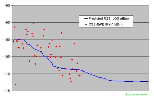
It can be observed that there is a correlation between the measured trend and the predicted trend in RSSI. Statistics calculation display the following results:
| Average error |
-1,4 dB |
| Stdev |
4,2dB |
2-ray for line of sight in Normal mode
In this graph the model is set to use a '2-ray model in Normal mode'
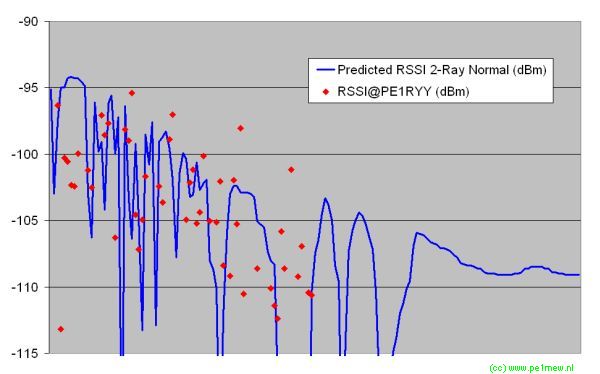
It can be observed that there is a correlation between the measured trend and the predicted trend in RSSI. However in this case very deep dips are predicted which are not found in reality.
Statistics calculation display the following results:
| Average error |
-1,8 dB |
| Stdev |
8,88 dB |
2-ray for line of sight in Interference mode
In this graph the model is set to use a '2-ray model in Interference mode'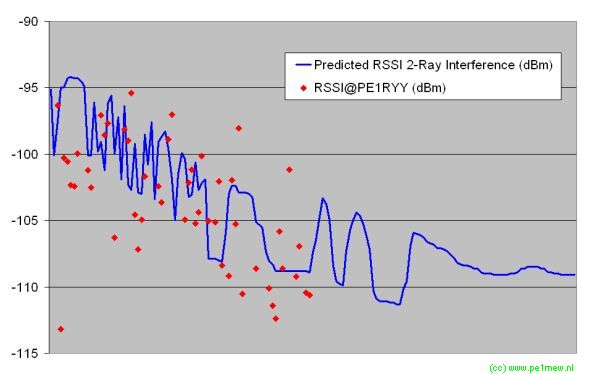
It can be observed that there is a correlation between the measured trend and the predicted trend in RSSI. Where in 'Normal mode' there are deep fading dips observed, in 'Interference mode' these seem to be delimited. Therefore the correlations seems stronger. Statistics calculation display the following results:
| Average error |
1,2dB |
| Stdev |
4,8dB |
All Predictions compared.
When all individual predictions are compared it can be seen that the there are generally two models and a third model that combines both:
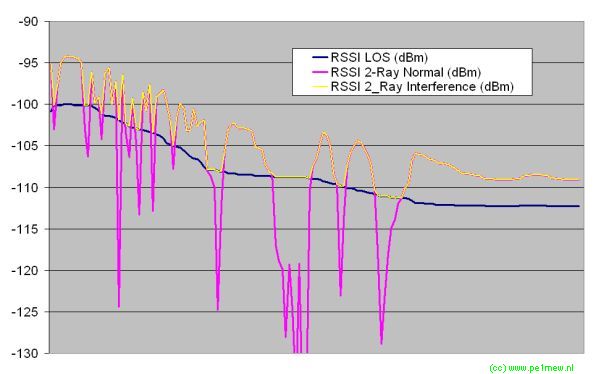
Model one is the 'No 2-ray for line of sight' type.
Model two is the '2-ray for line of sight in Normal mode'
Model three, 2-ray for line of sight in Interference mode, is a combination of both prior models. In this case when the predicted value in '2-ray for line of sight in Normal mode'< No 2-ray for line of sight' the value for that location is taken form the No 2-ray for line of sight' model.
2- Both visual check and mathematical verification
As the results of step one in the verification of the model was not very satisfying further investigation was started. This because some fading dips have been observed in de averaged RSSI data of PE1RYY.
Therefore both averaged RSSI data and predicted data was put in one graph.
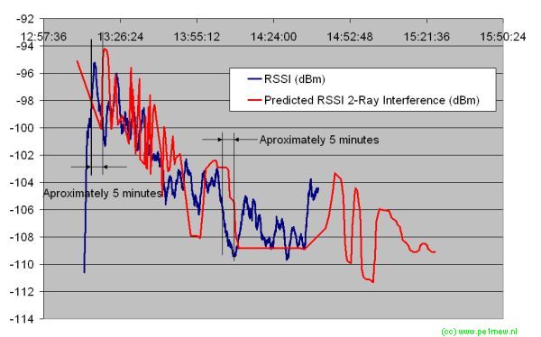
While studying this graph it was found that there was a correlation between the average RSSI and predicted RSSI but they seem to be shifted in time. Two checks (see above) learned that to the average RSSI had to be shifted 5 minutes in time and that probably the spectrum analyser atPE1RYY has it's clock 5 minutes earlier set.
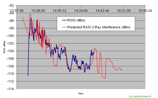
In the graph above the time correction of 5 minutes is applied.
To be able to do a mathematical analysis from both average RSSI and predicted RSSI the values are taken within a10 second window. This means that if in a 10 second window an measured and a predicted value are available they are assumed to have a relation and form a 'record'. Out of the 2 data sets 78 records have been taken.The analysis result shows that the 5 minute shift in time results in less average error and a better standard deviation:
| |
Without correction |
| Average error |
1,08dB |
| Stdev |
2,8dB |
Click on image for bigger one
|
| |
with 5 minutes correction |
| Average error |
-0,27dB |
| Stdev |
2,3dB |
Click on image for bigger one
|
Conclusion
Strong evidence has been found that ground reflections predicted by Radio Mobile occur in reality.
For the VHF frequency band the setting '2-ray for line of sight in Interference mode' gives best results and highest correlation.
The model '2-ray for line of sight in Normal mode' does not give accurate results while being used in air to ground communications. Therefore it is not advised to use.
As a good second choice the 'No 2-ray for line of sight' model gives sensible results.
Future improvements to measurements.
The next time this type of measurement will be performed some improvements have to be made:
- Timing is everything. All measurement equipment must be time synchronised. This can be done for example by using a GPS in combination with Tardis if localised synchronisation is required or over the internet when available.
- A increase of route points by the balloon is required. Compared by the large amount of survey data, 78records to be analysed is not much.
- Settings of the spectrum analyser have to be set better. By setting the spectrum analyser and recording PC better it mus be possible to determine the rotation speed of the balloon payload.
|


 Raw NMEA log file in ASCII text
 Excel file used for analysis and conversion
 Line object file created of the route.

