|
The accuracy of a model predicting RF propagation can be expressed in the following KPI (Key Performance Indicator):
- Average error of predicted to the measured fieldstrength
- Standard deviation
- Correlation of the predicted to the measured fieldstregth
The optical verification, where we will compare the prediction results with the survey data in a map window, will not produce results with the accuracy or numbers as suggested above.
The optical verification method is a rough, quick and dirty, way to determine if the result for the analysis makes sense. If you have experience in processing large tables in excel and know something about coordinate systems, dB's and fieldstrength calulation it is suggested to follow the mathematical appoach.
Verification example.
Before you can do a verification survey data has to be processed and ready for useage. Collecting data is described in 'Test site' and 'Survey vehicle'. Post processing survey data is described in 'Survey data'
The verification is done in general terain as can be found in the Netherlands. In 3 types of areas survey data is collected over a relative short distance (0.5 Km to 20 Km). The terrain types are:
- Forest areas with hilly terrain
- Urban areas
- Rural areas (general agricultural representative to the Netherlands)
The individual results per area are discribed below.
In this example the mode of variability is choosen to be 'mobile'. It is subject of discussion on what to choose. the mode of variability is described in 'ITM model propagation settings'
As a best practise, for amateurradio useage in a mobile environment best results are archived using the mode of availability setting: 'mobile'.
The following example displays the settings for VHF frequency's and wich are used for this verification.
However the frequencys used in the example are not in the 2 meter band they are close enough to this band to use the outcome for amateurradio use.
Preparations.
As the ITM model does not leave us many parameters to set, we leave them to the default value. The default values are displayed in the following image.
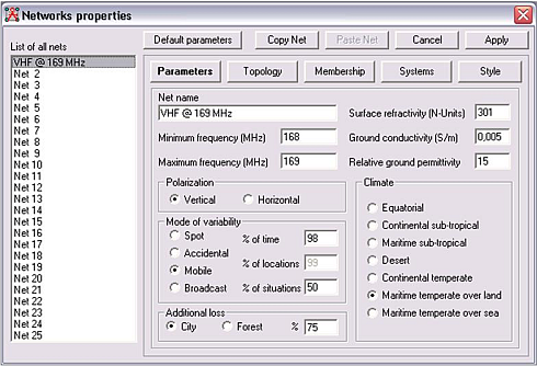
In this image you can see the settings I have been using for the test site. These settings must match exactly the transmitter configuration as it was installed for the test when the survey data was collected.
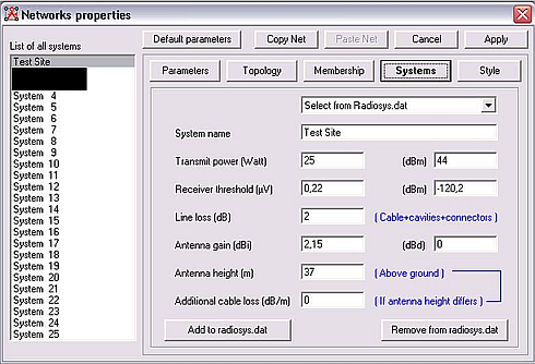
Some notes on Land cover
Radio mobile can do RF propagation predictions while taking in account Land cover (clutter).
In this verification example clutter is not evaluated. the results displays the outcome when using bare SRTM. If you want to evaluate the effect of clutter or include clutter, the mathematical verification must be applied.
To display the results of the survey data in Radio Mobile the function 'Load data > Use Cartasian Coverage' is used. See 'How to > Cartasian coverage > Load data' on how to perform this.
Forest area.
When the drivetest results with the fieldstrength measurements is imported in the map window you can see the route that has been driven.
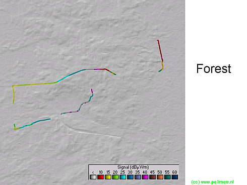
It is my objective not to have line of sight infulence my results. So I excluded parts of the results from the file. These are displayed in the following image.
To be able to 'tune' the model for forest areas the route was so choosen that only forest area is measured.
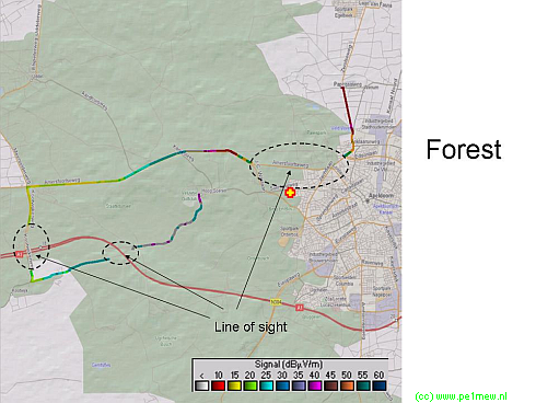
After importing the drivetest results it is essential that fieldstrength colors are set equally for both drivetest and prediction. When this is set properly it can be determined if the prediction equals the measurement. If this is the case we have a proper setting for the model.
In the following setting (T=98%, P=98%, F=0%) we see clearly that the prediction results do not match to the drivetest result as we can identify the route in the prediction result.
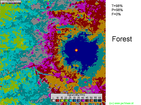
The drivetest data used is post processed. Due to fast and slow fading th signal has a lot of variation and to strip this out the data is 'Lee avaraged' The rusult of thi is that the drive test data represents 50% of place and > 95% of time. Because of this we have to set the model to equal values and we have to keep these fixed dring the tuning process.
The next step is to vary the Forrest compensation factor. I have done it in 25% steps. The following images display the results of this process.
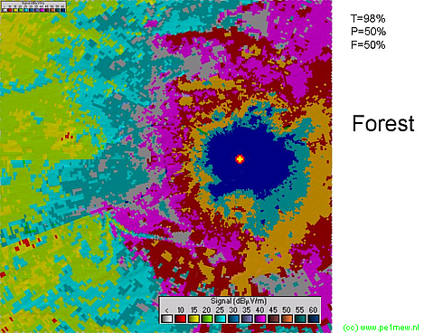
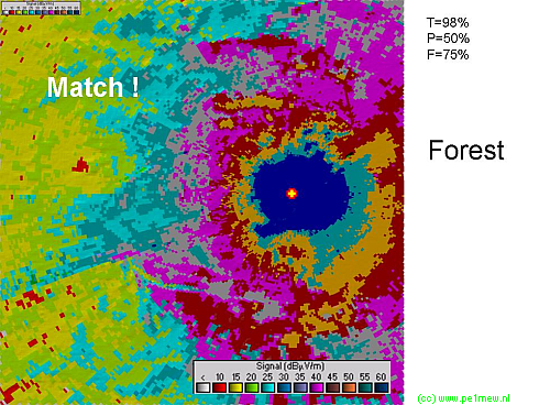
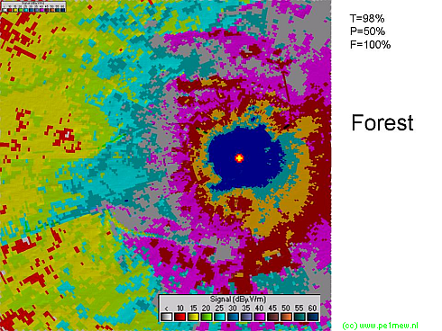
As you can see the forest compensation factor fits best to the drive test result at 75%.
Urban and rural areas
Here the results of a drivetest in urban and rural areas.
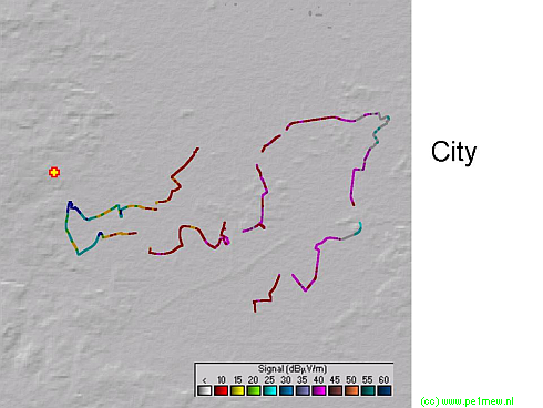
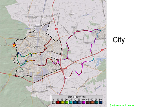
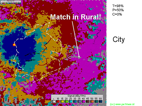
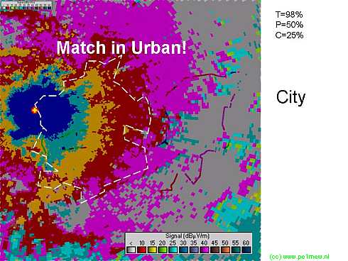
As you can see the city compensation factor in rural areas fits best to the drive test result at 0%. The city compensation factor in urban areas fits best to the drive test result at 25%
Best practise settings for VHF frequency's
| Variable |
value |
| % time |
98% for all areas |
| % place |
50% for all areas |
| % Forest correction |
Forest areas 75% |
| % City correction |
Urban areas 25%
Rural areas 0% |
|